import pandas as pd

# Load the data into a variable called 'df' (short for DataFrame)
# If you renamed your file, change the name inside the quotes below
filename = 'Респонденты, балюусь со временем - Ответы на форму (1)-3.csv'
df = pd.read_csv(filename)

# .shape tells us the size of the data (rows, columns)
print(f"Data Loaded Successfully!")
print(f"Rows: {df.shape[0]}, Columns: {df.shape[1]}")

# .head() shows the first 5 rows so we can visually check it
df.head()
Data Loaded Successfully!
Rows: 206, Columns: 75
| Отметка времени | Я ... | Мне ... | Какие устройства у меня имеются (можно выбрать несколько) | В среднем в будний день я провожу перед экраном ... | Наш расчет ср нед | В среднем в выходной день я провожу перед экраном ... | Наш расчет ср вых | Сколько у вас экранного времени было вчера? | Сколько у вас экранного времени было позавчера? | ... | Малина – ягода.1 | Отравление – смерть | Малина – ягода.2 | Враг – неприятель.3 | Отравление – смерть.1 | Враг – неприятель.4 | Море – океан.2 | Отравление – смерть.2 | Свет – темнота.2 | Итог | |
|---|---|---|---|---|---|---|---|---|---|---|---|---|---|---|---|---|---|---|---|---|---|
| 0 | 14.12.2024 15:14:38 | Девочка | 15 лет | Планшет | 12 | 12 | 12 | 12 | 12 | 12 | ... | 0.0 | 0.0 | 0.0 | 0.0 | 0.0 | 0.0 | 0.0 | 0.0 | 0.0 | 1.0 |
| 1 | 14.12.2024 15:18:18 | Девочка | 15 лет | Смартфон, Компьютер|Ноутбук | 3 | 4 | 5 | 3,5 | 3 | 4 | ... | 1.0 | 0.0 | 0.0 | 0.0 | 0.0 | 0.0 | 0.0 | 0.0 | 0.0 | 3.0 |
| 2 | 14.12.2024 15:19:44 | Мальчик | 15 лет | Смартфон, Компьютер|Ноутбук | 7 | 6 | 3 | 11 | 12 | 10 | ... | 0.0 | 0.0 | 1.0 | 1.0 | 0.0 | 0.0 | 1.0 | 0.0 | 0.0 | 5.0 |
| 3 | 14.12.2024 15:24:39 | Девочка | 15 лет | Смартфон, Компьютер|Ноутбук | 3 | 3,8 | 6 | 4 | 3 | 5 | ... | 0.0 | 0.0 | 0.0 | 1.0 | 0.0 | 0.0 | 0.0 | 0.0 | 0.0 | 3.0 |
| 4 | 14.12.2024 15:24:44 | Девочка | 15 лет | Смартфон, Компьютер|Ноутбук | 5 | 7 | 7 | 5 | 6 | 4 | ... | 0.0 | 0.0 | 1.0 | 1.0 | 0.0 | 1.0 | 1.0 | 0.0 | 0.0 | 5.0 |
5 rows × 75 columns
# 1. Rename difficult columns to simple variables
# This mapping focuses on the most important statistical columns
new_names = {
    'Я ...': 'Gender',
    'Мне ...': 'Age',
    'В среднем в будний день я провожу перед экраном ...': 'ScreenTime_Weekday',
    'В среднем в выходной день я провожу перед экраном ...': 'ScreenTime_Weekend',
    'Какая у тебя средняя оценка по всем предметам': 'GPA',
    'Сколько часов ты в среднем спишь?': 'Sleep_Hours',
    'Итог': 'Total_Score' # Psychometric score
}

df = df.rename(columns=new_names)

# 2. Remove completely empty rows
df = df.dropna(how='all')

# 3. Function to clean numbers (change "3,5" to 3.5)
def clean_currency_format(x):
    if pd.isna(x):
        return None
    # Convert to string, replace comma with dot
    x_str = str(x).replace(',', '.')
    # Extract only the number part (removes " лет" or other text)
    try:
        import re
        # This regex looks for numbers, possibly with decimals
        number = re.findall(r"[-+]?\d*\.\d+|\d+", x_str)
        if number:
            return float(number[0])
        return None
    except:
        return None

# List of columns that need to be numbers
numeric_cols = ['Age', 'ScreenTime_Weekday', 'ScreenTime_Weekend', 'GPA', 'Sleep_Hours', 'Total_Score']

# Apply the cleaning function to these columns
for col in numeric_cols:
    df[col] = df[col].apply(clean_currency_format)

# Check the results
print("Data Cleaned!")
print("Here is the data type information (Look for 'float64'):")
print("-" * 30)
df[numeric_cols].info()

# Show the first few rows to verify decimals look correct (e.g., 3.5 instead of 3,5)
df[numeric_cols].head()
Data Cleaned!
Here is the data type information (Look for 'float64'):
------------------------------
<class 'pandas.core.frame.DataFrame'>
Index: 188 entries, 0 to 205
Data columns (total 6 columns):
# Column Non-Null Count Dtype
--- ------ -------------- -----
0 Age 187 non-null float64
1 ScreenTime_Weekday 188 non-null float64
2 ScreenTime_Weekend 188 non-null float64
3 GPA 184 non-null float64
4 Sleep_Hours 187 non-null float64
5 Total_Score 187 non-null float64
dtypes: float64(6)
memory usage: 10.3 KB
| Age | ScreenTime_Weekday | ScreenTime_Weekend | GPA | Sleep_Hours | Total_Score | |
|---|---|---|---|---|---|---|
| 0 | 15.0 | 12.0 | 12.0 | 3.27 | 3.0 | 1.0 |
| 1 | 15.0 | 3.0 | 5.0 | 4.61 | 8.0 | 3.0 |
| 2 | 15.0 | 7.0 | 3.0 | 4.01 | 6.0 | 5.0 |
| 3 | 15.0 | 3.0 | 6.0 | 4.23 | 6.0 | 3.0 |
| 4 | 15.0 | 5.0 | 7.0 | 3.94 | 6.0 | 5.0 |
# 1. Get a statistical summary of the main columns
stats_summary = df[['Age', 'GPA', 'Sleep_Hours', 'ScreenTime_Weekday', 'ScreenTime_Weekend', 'Total_Score']].describe()

# 2. Round to 2 decimal places for easier reading
display(stats_summary.round(2))| Age | GPA | Sleep_Hours | ScreenTime_Weekday | ScreenTime_Weekend | Total_Score | |
|---|---|---|---|---|---|---|
| count | 187.00 | 184.00 | 187.00 | 188.00 | 188.00 | 187.00 |
| mean | 14.60 | 4.13 | 6.68 | 5.77 | 7.51 | 3.14 |
| std | 0.92 | 0.55 | 1.35 | 2.98 | 3.99 | 1.64 |
| min | 13.00 | 0.00 | 2.00 | 1.00 | 1.00 | 0.00 |
| 25% | 14.00 | 3.81 | 6.00 | 4.00 | 5.00 | 2.00 |
| 50% | 14.00 | 4.10 | 7.00 | 6.00 | 7.00 | 3.00 |
| 75% | 15.00 | 4.50 | 8.00 | 7.00 | 10.00 | 4.00 |
| max | 17.00 | 6.00 | 10.00 | 20.00 | 24.00 | 9.00 |
# 1. Check how many rows we have before filtering
print(f"Original Row Count: {len(df)}")

# 2. Apply Filters
# Keep GPA <= 5
df = df[df['GPA'] <= 5]

# Keep Time variables <= 24 hours (Physical limit)
df = df[df['Sleep_Hours'] <= 24]
df = df[df['ScreenTime_Weekday'] <= 24]
df = df[df['ScreenTime_Weekend'] <= 24]

# 3. Check how many rows remain
print(f"Row Count after cleaning outliers: {len(df)}")

# 4. Show the new descriptive statistics to confirm the Max values are fixed
clean_stats = df[['GPA', 'Sleep_Hours', 'ScreenTime_Weekday', 'ScreenTime_Weekend']].describe()
display(clean_stats.round(2))
Original Row Count: 188
Row Count after cleaning outliers: 183
| GPA | Sleep_Hours | ScreenTime_Weekday | ScreenTime_Weekend | |
|---|---|---|---|---|
| count | 183.00 | 183.00 | 183.00 | 183.00 |
| mean | 4.12 | 6.68 | 5.75 | 7.51 |
| std | 0.53 | 1.35 | 3.00 | 4.01 |
| min | 0.00 | 2.00 | 1.00 | 1.00 |
| 25% | 3.81 | 6.00 | 4.00 | 5.00 |
| 50% | 4.09 | 7.00 | 6.00 | 7.00 |
| 75% | 4.49 | 8.00 | 7.00 | 10.00 |
| max | 5.00 | 10.00 | 20.00 | 24.00 |
import matplotlib.pyplot as plt
import seaborn as sns

# 1. Numeric Comparison Table
# We group the data by 'Gender' and calculate the median for key columns
gender_stats = df.groupby('Gender')[['ScreenTime_Weekday', 'ScreenTime_Weekend', 'GPA', 'Sleep_Hours']].mean()
print("Average (Mean) Values by Gender:")
display(gender_stats.round(2))

# 2. Visual Comparison (Boxplots)
# We will create 2 side-by-side plots: one for Weekend Screen Time, one for GPA
fig, axes = plt.subplots(1, 2, figsize=(14, 6))

# Plot A: Screen Time on Weekends
sns.boxplot(data=df, x='Gender', y='ScreenTime_Weekend', palette="pastel", ax=axes[0])
axes[0].set_title('Screen Time: Weekends')
axes[0].set_ylabel('Hours')

# Plot B: GPA (Grades)
sns.boxplot(data=df, x='Gender', y='GPA', palette="pastel", ax=axes[1])
axes[1].set_title('Academic Performance (GPA)')
axes[1].set_ylabel('Grade (1-5)')

plt.tight_layout()
plt.show()
Average (Mean) Values by Gender:
| ScreenTime_Weekday | ScreenTime_Weekend | GPA | Sleep_Hours | |
|---|---|---|---|---|
| Gender | ||||
| Девочка | 5.77 | 7.47 | 4.19 | 6.36 |
| Мальчик | 5.71 | 7.58 | 4.00 | 7.21 |
/var/folders/d8/4k3q_2wd4nv9gmh9ch_b79jr0000gn/T/ipykernel_11930/2536227559.py:15: FutureWarning:

Passing `palette` without assigning `hue` is deprecated and will be removed in v0.14.0. Assign the `x` variable to `hue` and set `legend=False` for the same effect.

  sns.boxplot(data=df, x='Gender', y='ScreenTime_Weekend', palette="pastel", ax=axes[0])
/var/folders/d8/4k3q_2wd4nv9gmh9ch_b79jr0000gn/T/ipykernel_11930/2536227559.py:20: FutureWarning:

Passing `palette` without assigning `hue` is deprecated and will be removed in v0.14.0. Assign the `x` variable to `hue` and set `legend=False` for the same effect.

  sns.boxplot(data=df, x='Gender', y='GPA', palette="pastel", ax=axes[1])

# Select only the columns we care about for relationships
cols_for_corr = ['Age', 'ScreenTime_Weekday', 'ScreenTime_Weekend', 'GPA', 'Sleep_Hours', 'Total_Score']

# Calculate the correlation matrix
corr_matrix = df[cols_for_corr].corr()

# Plot the Heatmap
plt.figure(figsize=(10, 8))
sns.heatmap(corr_matrix,
            annot=True,      # Show the numbers on the squares
            cmap='coolwarm', # Blue for negative, Red for positive
            vmin=-1, vmax=1, # Fix the scale from -1 to 1
            fmt=".2f")       # Show 2 decimal places

plt.title('Correlation Map: What affects what?')
plt.show()
import matplotlib.pyplot as plt
import seaborn as sns

# Create the Scatter Plot with Regression Lines
# height and aspect control the size of the image
grid = sns.lmplot(
    data=df,
    x='ScreenTime_Weekend',  # The Cause (Independent Variable)
    y='GPA',                 # The Effect (Dependent Variable)
    hue='Gender',            # Different colors for Boys/Girls
    height=6,
    aspect=1.5,
    scatter_kws={'alpha': 0.6, 's': 50}, # Make dots semi-transparent and larger
    line_kws={'linewidth': 3}            # Make the trend lines thick
)

# Customizing the chart for your report
plt.title('Impact of Weekend Screen Time on GPA', fontsize=16)
plt.xlabel('Screen Time (Hours/Day on Weekend)', fontsize=12)
plt.ylabel('GPA (Grade 1-5)', fontsize=12)

# Set limits to focus on the relevant data area
plt.ylim(2.5, 5.2)  # Focus on passing grades up to max
plt.xlim(0, 24)     # 0 to 24 hours

plt.show()
# 1. Split the data into two groups
boys_data = df[df['Gender'] == 'Мальчик']
girls_data = df[df['Gender'] == 'Девочка']

# 2. Calculate the specific correlation for each group
# We look at Weekend Screen Time vs GPA
r_boys = boys_data['ScreenTime_Weekend'].corr(boys_data['GPA'])
r_girls = girls_data['ScreenTime_Weekend'].corr(girls_data['GPA'])

# 3. Print the results
print("-" * 30)
print(f"Impact of Screen Time on Grades (Correlation 'r'):")
print("-" * 30)
print(f"Boys:  {r_boys:.3f}  ( steeper slope / stronger effect )")
print(f"Girls: {r_girls:.3f}  ( flatter slope / weaker effect )")
print("-" * 30)

if abs(r_boys) > abs(r_girls):
    print("CONCLUSION: You were right. The negative trend is stronger for boys.")
else:
    print("CONCLUSION: The trend is actually similar, despite the visual.")
---------------------------------------------------------------------------
NameError Traceback (most recent call last)
Cell In[2], line 2
1 # 1. Split the data into two groups
----> 2 boys_data = df[df['Gender'] == 'Мальчик']
3 girls_data = df[df['Gender'] == 'Девочка']
5 # 2. Calculate the specific correlation for each group
6 # We look at Weekend Screen Time vs GPA
NameError: name 'df' is not defined
import pandas as pd
import numpy as np
import re

# --- RELOAD AND CLEAN DATA ---
filename = 'Респонденты, балюусь со временем - Ответы на форму (1)-3.csv'
df = pd.read_csv(filename)

# Rename columns
new_names = {
    'Я ...': 'Gender',
    'Мне ...': 'Age',
    'В среднем в будний день я провожу перед экраном ...': 'ScreenTime_Weekday',
    'В среднем в выходной день я провожу перед экраном ...': 'ScreenTime_Weekend',
    'Какая у тебя средняя оценка по всем предметам': 'GPA',
    'Сколько часов ты в среднем спишь?': 'Sleep_Hours',
    'Итог': 'Total_Score'
}
df = df.rename(columns=new_names)

# Remove empty rows
df = df.dropna(how='all')

# Function to fix "3,5" -> 3.5
def clean_currency_format(x):
    if pd.isna(x): return None
    x_str = str(x).replace(',', '.')
    try:
        number = re.findall(r"[-+]?\d*\.\d+|\d+", x_str)
        return float(number[0]) if number else None
    except: return None

# Apply cleaning
numeric_cols = ['Age', 'ScreenTime_Weekday', 'ScreenTime_Weekend', 'GPA', 'Sleep_Hours', 'Total_Score']
for col in numeric_cols:
    df[col] = df[col].apply(clean_currency_format)

# Remove Outliers (sanity check)
df = df[df['GPA'] <= 5]
df = df[df['Sleep_Hours'] <= 24]
df = df[df['ScreenTime_Weekday'] <= 24]
df = df[df['ScreenTime_Weekend'] <= 24]

# --- NEW ANALYSIS: BOYS vs GIRLS CORRELATION ---

# 1. Split the data
boys_data = df[df['Gender'] == 'Мальчик']
girls_data = df[df['Gender'] == 'Девочка']

# 2. Calculate correlations
r_boys = boys_data['ScreenTime_Weekend'].corr(boys_data['GPA'])
r_girls = girls_data['ScreenTime_Weekend'].corr(girls_data['GPA'])

# 3. Print Results
print("-" * 30)
print(f"Impact of Screen Time on Grades (Correlation 'r'):")
print("-" * 30)
print(f"Boys:  {r_boys:.3f}")
print(f"Girls: {r_girls:.3f}")
print("-" * 30)

if abs(r_boys) > abs(r_girls):
    print("CONCLUSION: You were right. The negative trend is stronger for boys.")
else:
    print("CONCLUSION: The trend is statistically similar or stronger for girls.")
------------------------------
Impact of Screen Time on Grades (Correlation 'r'):
------------------------------
Boys: -0.120
Girls: -0.325
------------------------------
CONCLUSION: The trend is statistically similar or stronger for girls.
import matplotlib.pyplot as plt
import seaborn as sns

# Create the Bar Chart
plt.figure(figsize=(8, 6))
sns.barplot(data=df, x='User_Group', y='Total_Score', hue='User_Group', palette='viridis')

plt.title('Cognitive Test Scores: Light vs. Heavy Screen Users')
plt.ylabel('Average Test Score')
plt.xlabel('User Category (Based on 7 hours split)')
plt.show()
from scipy.stats import mannwhitneyu

# 1. Separate the scores into two lists
scores_light = df[df['User_Group'] == 'Light User']['Total_Score']
scores_heavy = df[df['User_Group'] == 'Heavy User']['Total_Score']

# 2. Run the Test
stat, p_value = mannwhitneyu(scores_light, scores_heavy)

# 3. Print the Result clearly
print("-" * 40)
print(f"P-Value: {p_value:.4f}")
print("-" * 40)

if p_value < 0.05:
    print("VERDICT: The difference is REAL (Statistically Significant).")
    print("Screen time likely negatively affects the test score.")
else:
    print("VERDICT: The difference is NOT statistically significant.")
    print("The score difference (3.26 vs 3.09) is small enough that it could just be random chance.")
    print("We cannot prove screen time lowers cognitive scores based on this data.")
----------------------------------------
P-Value: 0.5184
----------------------------------------
VERDICT: The difference is NOT statistically significant.
The score difference (3.26 vs 3.09) is small enough that it could just be random chance.
We cannot prove screen time lowers cognitive scores based on this data.
from scipy.stats import mannwhitneyu

# 1. Compare Sleep Hours between Heavy (>7h) and Light (<7h) users
sleep_light = df[df['User_Group'] == 'Light User']['Sleep_Hours']
sleep_heavy = df[df['User_Group'] == 'Heavy User']['Sleep_Hours']

# 2. Calculate the average sleep for context
print(f"Average Sleep (Light Users): {sleep_light.mean():.2f} hours")
print(f"Average Sleep (Heavy Users): {sleep_heavy.mean():.2f} hours")

# 3. Run the Statistical Test
stat, p_value = mannwhitneyu(sleep_light, sleep_heavy)

print("-" * 40)
print(f"P-Value: {p_value:.4f}")
print("-" * 40)

if p_value < 0.05:
    print("VERDICT: SIGNIFICANT DIFFERENCE FOUND!")
    print("We can scientifically prove that heavy screen users get less sleep.")
else:
    print("VERDICT: No significant difference.")
Average Sleep (Light Users): 6.88 hours
Average Sleep (Heavy Users): 6.42 hours
----------------------------------------
P-Value: 0.0552
----------------------------------------
VERDICT: No significant difference.
# 1. Rename the long question column
# "Как ты думаешь время перед экраном влияет на твой сон (хуже или лучше)?"
col_name_subjective = 'Как ты думаешь время перед экраном влияет на твой сон (хуже или лучше)?'
df = df.rename(columns={col_name_subjective: 'Opinion_Sleep'})

# 2. Check what answers students gave
print("Student Opinions on Screen Time & Sleep:")
print(df['Opinion_Sleep'].value_counts())

# 3. Visualize Actual Sleep vs. Their Opinion
plt.figure(figsize=(10, 6))
sns.boxplot(data=df, x='Opinion_Sleep', y='Sleep_Hours', palette='Set2')

plt.title('Self-Awareness: Opinion vs. Actual Sleep')
plt.xlabel('Student Opinion: "Does screen time affect your sleep?"')
plt.ylabel('Actual Sleep (Hours)')
plt.show()

# 4. Calculate the average sleep for each opinion group
print("-" * 30)
print("Actual Average Sleep by Opinion Group:")
print(df.groupby('Opinion_Sleep')['Sleep_Hours'].mean().round(2))
Student Opinions on Screen Time & Sleep:
Opinion_Sleep
Да 76
Нет 73
Не знаю 34
Name: count, dtype: int64
/var/folders/d8/4k3q_2wd4nv9gmh9ch_b79jr0000gn/T/ipykernel_13950/389020546.py:12: FutureWarning:
Passing `palette` without assigning `hue` is deprecated and will be removed in v0.14.0. Assign the `x` variable to `hue` and set `legend=False` for the same effect.
sns.boxplot(data=df, x='Opinion_Sleep', y='Sleep_Hours', palette='Set2')

------------------------------
Actual Average Sleep by Opinion Group:
Opinion_Sleep
Да         6.58
Не знаю    6.65
Нет        6.79
Name: Sleep_Hours, dtype: float64
import matplotlib.pyplot as plt
import seaborn as sns

plt.figure(figsize=(10, 6))

# 1. Determine the order (Highest median screen time on left)
order = df.groupby('App_Category')['ScreenTime_Weekend'].median().sort_values(ascending=False).index

# 2. Plot with the fix (hue=App_Category)
sns.boxplot(
    data=df,
    x='App_Category',
    y='ScreenTime_Weekend',
    order=order,
    hue='App_Category', # This fixes the warning
    palette='magma',
    legend=False
)

plt.title('Which App Users have the Highest Weekend Screen Time?')
plt.ylabel('Hours on Screen')
plt.show()
# 1. Rename the App column
col_app = 'Какое приложение на твоем смартфоне является рекордсменом по экранному времени?'
df = df.rename(columns={col_app: 'Top_App'})

# 2. Function to clean text (Combine "tik tok", "tt", "tiktok" into one)
def clean_app_name(text):
    if pd.isna(text): return "Unknown"
    text = str(text).lower().strip() # Make lowercase

    # Common mappings
    if 'tik' in text or 'tt' in text or 'тик' in text:
        return 'TikTok'
    if 'tele' in text or 'tg' in text or 'тг' in text:
        return 'Telegram'
    if 'tube' in text or 'ютуб' in text:
        return 'YouTube'
    if 'game' in text or 'игр' in text or 'brawl' in text or 'genshin' in text or 'pubg' in text:
        return 'Games'
    if 'whats' in text or 'vk' in text or 'вк' in text:
        return 'Social/Chat'

    return 'Other' # For browsers, maps, etc.

# Apply cleaning
df['App_Category'] = df['Top_App'].apply(clean_app_name)

# 3. View the Most Popular Apps
print("Most Popular Time-Wasting Apps:")
print(df['App_Category'].value_counts())

# 4. Visualization: Who spends the most time?
plt.figure(figsize=(10, 6))
# Sort order: Apps with highest median screen time on the left
order = df.groupby('App_Category')['ScreenTime_Weekend'].median().sort_values(ascending=False).index

sns.boxplot(data=df, x='App_Category', y='ScreenTime_Weekend', order=order, palette='magma')
plt.title('Which App Users have the Highest Weekend Screen Time?')
plt.ylabel('Hours on Screen')
plt.show()
Most Popular Time-Wasting Apps:
App_Category
TikTok 59
Telegram 53
Other 39
YouTube 25
Games 5
Unknown 2
Name: count, dtype: int64
/var/folders/d8/4k3q_2wd4nv9gmh9ch_b79jr0000gn/T/ipykernel_13950/3147444248.py:36: FutureWarning:
Passing `palette` without assigning `hue` is deprecated and will be removed in v0.14.0. Assign the `x` variable to `hue` and set `legend=False` for the same effect.
sns.boxplot(data=df, x='App_Category', y='ScreenTime_Weekend', order=order, palette='magma')

# Calculate the average (mean) weekend screen time for the top apps
app_stats = df.groupby('App_Category')['ScreenTime_Weekend'].mean().sort_values(ascending=False)

print("Average Weekend Screen Time by App (Hours):")
print("-" * 40)
print(app_stats)
print("-" * 40)

tiktok_avg = app_stats['TikTok']
telegram_avg = app_stats['Telegram']
diff = tiktok_avg - telegram_avg

print(f"CONCLUSION: TikTok users spend, on average, {diff:.2f} more hours per day")
print("on screens compared to Telegram users.")
Average Weekend Screen Time by App (Hours):
----------------------------------------
App_Category
Unknown 9.500000
TikTok 7.897119
Other 7.653846
Telegram 7.160377
YouTube 7.080000
Games 6.940000
Name: ScreenTime_Weekend, dtype: float64
----------------------------------------
CONCLUSION: TikTok users spend, on average, 0.74 more hours per day
on screens compared to Telegram users.
## We have switched to sleep and GPAimport matplotlib.pyplot as plt
import seaborn as sns
# Create the Scatter Plot with a Trend Line
sns.lmplot(
data=df,
x='Sleep_Hours',
y='GPA',
hue='Gender', # Let's keep looking if boys/girls differ
height=6,
aspect=1.5,
scatter_kws={'alpha': 0.6, 's': 50},
line_kws={'linewidth': 3}
)
plt.title('Does Sleeping More Equal Better Grades?', fontsize=16)
plt.xlabel('Average Sleep (Hours)', fontsize=12)
plt.ylabel('GPA (Grade 1-5)', fontsize=12)
plt.ylim(2.5, 5.2) # Focus on the passing grades
plt.show()
# 1. Split the data
boys_data = df[df['Gender'] == 'Мальчик']
girls_data = df[df['Gender'] == 'Девочка']

# 2. Calculate correlation: SLEEP vs GPA
r_boys_sleep = boys_data['Sleep_Hours'].corr(boys_data['GPA'])
r_girls_sleep = girls_data['Sleep_Hours'].corr(girls_data['GPA'])

# 3. Print the results
print("-" * 40)
print(f"Impact of Sleep on Grades (Correlation 'r'):")
print("-" * 40)
print(f"Boys:  {r_boys_sleep:.3f}")
print(f"Girls: {r_girls_sleep:.3f}")
print("-" * 40)

# Logic to interpret the result automatically
if r_boys_sleep > r_girls_sleep:
    print("CONCLUSION: You were right! Sleep is more critical for Boys' grades.")
else:
    print("CONCLUSION: Actually, sleep affects Girls' grades more (despite the graph).")
----------------------------------------
Impact of Sleep on Grades (Correlation 'r'):
----------------------------------------
Boys: 0.100
Girls: 0.168
----------------------------------------
CONCLUSION: Actually, sleep affects Girls' grades more (despite the graph).
import matplotlib.pyplot as plt
import seaborn as sns

# 1. Filter for the two big giants: TikTok and Telegram
# (We exclude "Other" or "Games" because they have fewer people)
target_apps = ['TikTok', 'Telegram']
app_sleep_data = df[df['App_Category'].isin(target_apps)]

# 2. Calculate average sleep for each
print("Average Sleep Hours by App:")
print("-" * 30)
print(app_sleep_data.groupby('App_Category')['Sleep_Hours'].mean().round(2))
print("-" * 30)

# 3. Visualize
plt.figure(figsize=(8, 6))
sns.barplot(
    data=app_sleep_data,
    x='App_Category',
    y='Sleep_Hours',
    palette='coolwarm',
    hue='App_Category' # Fixes the warning
)

plt.title('Do TikTok Users Sleep Less than Telegram Users?')
plt.ylabel('Average Sleep (Hours)')
plt.ylim(0, 9) # Set limit to see the bars clearly
plt.show()
Average Sleep Hours by App:
------------------------------
App_Category
Telegram 6.45
TikTok 6.58
Name: Sleep_Hours, dtype: float64
------------------------------

# 1. Rename the long column
col_sports = 'Сколько раз в неделю ты ходишь на тренировки?'
df = df.rename(columns={col_sports: 'Training_Freq'})

# 2. Check the categories
# We expect values like "Нет", "1-2", "2-3", "Более 3 раз"
print("Training Categories found:")
print(df['Training_Freq'].unique())

# 3. Calculate Average Sleep by Training Frequency
# We sort the values so the chart makes sense (None -> Low -> High)
order_list = ['Ни одного', 'Нет', '1-2', '2-3', 'Более 3 раз']

# Note: Your data might use "Нет" or "Ни одного" or "Ничего".
# The code below groups by whatever text is there.
sleep_by_sports = df.groupby('Training_Freq')['Sleep_Hours'].mean().sort_values()

print("-" * 30)
print("Does Sport help Sleep?")
print(sleep_by_sports)
print("-" * 30)

# 4. Visualize
plt.figure(figsize=(10, 6))
sns.boxplot(
    data=df,
    x='Training_Freq',
    y='Sleep_Hours',
    palette='Greens',
    hue='Training_Freq',
    order=['Нет', 'Ни одного', '1-2', '2-3', 'Более 3 раз'] # Trying to force a logical order
)

plt.title('Physical Training vs. Sleep Duration')
plt.ylabel('Hours of Sleep')
plt.xlabel('Training Frequency (Per Week)')
plt.show()
Training Categories found:
['2-3' '1-2' 'Ни одного' 'Более 3 раз' nan]
------------------------------
Does Sport help Sleep?
Training_Freq
1-2 6.534884
Ни одного 6.597826
Более 3 раз 6.629630
2-3 6.986842
Name: Sleep_Hours, dtype: float64
------------------------------

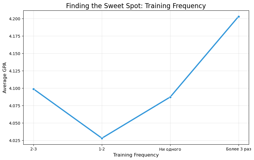
# 1. Calculate Average GPA by Training Frequency
gpa_by_sports = df.groupby('Training_Freq')['GPA'].mean().reindex(['Ни одного', '1-2', '2-3', 'Более 3 раз'])

print("-" * 30)
print("Does Sport help Grades?")
print(gpa_by_sports.round(2))
print("-" * 30)

# 2. Visualize
plt.figure(figsize=(10, 6))
sns.barplot(
    data=df,
    x='Training_Freq',
    y='GPA',
    palette='Greens',
    order=['Ни одного', '1-2', '2-3', 'Более 3 раз'],
    ci=None # Remove error bars for a cleaner look at the mean
)

plt.title('Physical Training vs. Academic Performance (GPA)')
plt.ylabel('Average GPA')
plt.xlabel('Training Frequency (Per Week)')
plt.ylim(3.5, 4.5) # Zoom in to see the difference
plt.show()
------------------------------
Does Sport help Grades?
Training_Freq
Ни одного 4.09
1-2 4.03
2-3 4.10
Более 3 раз 4.20
Name: GPA, dtype: float64
------------------------------
/var/folders/d8/4k3q_2wd4nv9gmh9ch_b79jr0000gn/T/ipykernel_13950/3034588233.py:11: FutureWarning:
The `ci` parameter is deprecated. Use `errorbar=None` for the same effect.
sns.barplot(
/var/folders/d8/4k3q_2wd4nv9gmh9ch_b79jr0000gn/T/ipykernel_13950/3034588233.py:11: FutureWarning:
Passing `palette` without assigning `hue` is deprecated and will be removed in v0.14.0. Assign the `x` variable to `hue` and set `legend=False` for the same effect.
sns.barplot(

from scipy.stats import mannwhitneyu

# 1. Isolate the two groups
# Group A: The "Sweet Spot" (2-3 times a week)
sleep_peak = df[df['Training_Freq'] == '2-3']['Sleep_Hours']

# Group B: The "Casual" group (1-2 times a week)
sleep_low = df[df['Training_Freq'] == '1-2']['Sleep_Hours']

# 2. Print the averages again to be sure
print(f"Average Sleep (2-3 times): {sleep_peak.mean():.2f} hours")
print(f"Average Sleep (1-2 times): {sleep_low.mean():.2f} hours")
print("-" * 40)

# 3. Run the P-Value Test
stat, p_value = mannwhitneyu(sleep_peak, sleep_low)

print(f"P-Value: {p_value:.4f}")
print("-" * 40)

# 4. Interpretation
if p_value < 0.05:
    print("VERDICT: SIGNIFICANT.")
    print("The increase in sleep for the '2-3 times' group is REAL.")
elif p_value < 0.10:
    print("VERDICT: MARGINALLY SIGNIFICANT (Trend).")
    print("There is a strong signal, but not quite 95% certainty.")
else:
    print("VERDICT: NOT SIGNIFICANT.")
    print("This is likely just a fluctuation.")
Average Sleep (2-3 times): 6.99 hours
Average Sleep (1-2 times): 6.53 hours
----------------------------------------
P-Value: 0.0407
----------------------------------------
VERDICT: SIGNIFICANT.
The increase in sleep for the '2-3 times' group is REAL.
from scipy.stats import spearmanr

# 1. Clean the data (Drop any rows where Sleep or GPA is missing)
clean_data = df.dropna(subset=['Sleep_Hours', 'GPA'])

# 2. Run the Spearman Correlation Test
# This checks if there is a monotonic relationship (as one goes up, the other goes up)
coef, p_value = spearmanr(clean_data['Sleep_Hours'], clean_data['GPA'])

print("-" * 40)
print(f"Correlation Coefficient (r): {coef:.3f}")
print(f"P-Value: {p_value:.4f}")
print("-" * 40)

# 3. Interpretation
if p_value < 0.05:
    print("VERDICT: SIGNIFICANT.")
    print("There is a REAL statistical link: More sleep = Higher Grades.")
    print("Even if the correlation is weak, it is not random luck.")
else:
    print("VERDICT: NOT SIGNIFICANT.")
    print("We cannot prove that sleep directly changes grades in this specific dataset.")
----------------------------------------
Correlation Coefficient (r): 0.060
P-Value: 0.4203
----------------------------------------
VERDICT: NOT SIGNIFICANT.
We cannot prove that sleep directly changes grades in this specific dataset.
import statsmodels.api as sm

# 1. Prepare the data
# We need rows that have data for ALL three columns
subset = df[['GPA', 'Sleep_Hours', 'ScreenTime_Weekend']].dropna()

# 2. Define Y (Target) and X (Predictors)
Y = subset['GPA']
X = subset[['Sleep_Hours', 'ScreenTime_Weekend']]

# Add a "Constant" (The baseline GPA if you did nothing) - required for the math to work
X = sm.add_constant(X)

# 3. Fit the Model (Ordinary Least Squares)
model = sm.OLS(Y, X).fit()

# 4. Print the "clean" results
print("--- COMBINED EFFECT ANALYSIS ---")
print(f"R-squared: {model.rsquared:.3f} (How much of the GPA is explained by these two?)")
print("-" * 50)
print(model.summary().tables[1])
print("-" * 50)
--- COMBINED EFFECT ANALYSIS ---
R-squared: 0.061 (How much of the GPA is explained by these two?)
--------------------------------------------------
======================================================================================
coef std err t P>|t| [0.025 0.975]
--------------------------------------------------------------------------------------
const 4.2364 0.222 19.087 0.000 3.798 4.674
Sleep_Hours 0.0172 0.029 0.594 0.553 -0.040 0.074
ScreenTime_Weekend -0.0313 0.010 -3.214 0.002 -0.051 -0.012
======================================================================================
--------------------------------------------------
# --- DATASET SUMMARY REPORT ---

# 1. Total Sample Size (N)
N = len(df)

# 2. Gender Breakdown
gender_counts = df['Gender'].value_counts()
gender_pct = df['Gender'].value_counts(normalize=True) * 100

# 3. Key Statistics (Mean +/- Standard Deviation)
avg_age = df['Age'].mean()
sd_age = df['Age'].std()

avg_gpa = df['GPA'].mean()
sd_gpa = df['GPA'].std()

avg_screen_wknd = df['ScreenTime_Weekend'].mean()
sd_screen_wknd = df['ScreenTime_Weekend'].std()

avg_sleep = df['Sleep_Hours'].mean()
sd_sleep = df['Sleep_Hours'].std()

# --- PRINT THE REPORT ---
print("="*40)
print("DATASET DEMOGRAPHIC SUMMARY")
print("="*40)
print(f"Total Participants (N): {N}")
print("-" * 40)
print("GENDER DISTRIBUTION:")
for gender in gender_counts.index:
    count = gender_counts[gender]
    pct = gender_pct[gender]
    print(f"  - {gender}: {count} ({pct:.1f}%)")
print("-" * 40)
print("DESCRIPTIVE STATISTICS (Mean ± SD):")
print(f"  - Age: {avg_age:.2f} ± {sd_age:.2f} years")
print(f"  - GPA: {avg_gpa:.2f} ± {sd_gpa:.2f}")
print(f"  - Weekend Screen Time: {avg_screen_wknd:.2f} ± {sd_screen_wknd:.2f} hours")
print(f"  - Sleep Duration: {avg_sleep:.2f} ± {sd_sleep:.2f} hours")
print("="*40)
========================================
DATASET DEMOGRAPHIC SUMMARY
========================================
Total Participants (N): 183
----------------------------------------
GENDER DISTRIBUTION:
- Девочка: 114 (62.3%)
- Мальчик: 69 (37.7%)
----------------------------------------
DESCRIPTIVE STATISTICS (Mean ± SD):
- Age: 14.62 ± 0.92 years
- GPA: 4.12 ± 0.53
- Weekend Screen Time: 7.51 ± 4.01 hours
- Sleep Duration: 6.68 ± 1.35 hours
========================================
# Save to CSV
# index=False tells Python not to save the row numbers (0, 1, 2...) as a column
df.to_csv('survey_data_cleaned.csv', index=False)

print("Success! File 'survey_data_cleaned.csv' has been saved to your folder.")
Success! File 'survey_data_cleaned.csv' has been saved to your folder.
# 1. Define the Answer Key Dictionary
# Key = Column Name in CSV, Value = The Correct Answer String
answer_key = {
    'Плакать – реветь*': 'Враг – неприятель',
    'Пара – два': 'Враг – неприятель',
    'Свобода – воля': 'Враг – неприятель',
    'Глава – роман': 'Овца – стадо',
    'Страна – город': 'Овца – стадо',
    'Покой – движение': 'Свет – темнота',
    'Похвала – брань': 'Свет – темнота',
    'Тумбочка – шкаф': 'Море – океан',
    'Химия – наука': 'Малина – ягода',
    'Грядка – огород': 'Овца – стадо',
    'Буква – слово': 'Овца – стадо',
    'Пение – искусство': 'Малина – ягода',
    'Месть – поджог': 'Отравление – смерть', # Based on rubric mapping
    'Девять – число': 'Малина – ягода',
    'Правильно – верно': 'Враг – неприятель',
    'Обман – недоверие': 'Отравление – смерть',
    'Смелость – геройство': 'Море – океан',
    'Прохлада – мороз': 'Море – океан',
    'Испуг – бегство': 'Отравление – смерть',
    'Бодрый – вялый': 'Враг – неприятель' # Wait, 'Bodry-Vyaly' is Antonym -> Svet-Temnota?
}
# Correction based on logic: 'Бодрый – вялый' (Energetic - Lethargic) is Antonym.
# Logic dictates 'Свет – темнота'. Let's verify the key image.
# Key #7 (Бодрый – вялый) -> Г (Svet-Temnota).
# Updating dictionary:
answer_key['Бодрый – вялый'] = 'Свет – темнота'

# 2. Grading Function
def calculate_test_score(row):
    score = 0
    # Loop through each question
    for question, correct_answer in answer_key.items():
        # Check if the column exists (to avoid errors)
        if question in row:
            # Get student's answer, clean it (strip spaces)
            student_ans = str(row[question]).strip()
            if student_ans == correct_answer:
                score += 1
    return score

# 3. Apply Grading (Raw Score 0-20)
df['Raw_Cognitive_Score'] = df.apply(calculate_test_score, axis=1)

# 4. Convert to 1-9 Scale (Rubric)
def apply_scale(raw):
    if raw >= 19: return 9
    if raw == 18: return 8
    if raw == 17: return 7
    if raw >= 15: return 6
    if raw >= 12: return 5
    if raw >= 10: return 4
    if raw >= 8:  return 3
    if raw == 7:  return 2
    return 1

df['Scaled_Cognitive_Score'] = df['Raw_Cognitive_Score'].apply(apply_scale)

# 5. Check the Results
print("Grading Complete!")
print("Here is a sample of the new scores:")
display(df[['Raw_Cognitive_Score', 'Scaled_Cognitive_Score', 'Total_Score']].head(10))

# Compare Old Score vs New Score
correlation_check = df['Scaled_Cognitive_Score'].corr(df['Total_Score'])
print(f"\nCorrelation between your Old Score and New Calculated Score: {correlation_check:.2f}")
Grading Complete!
Here is a sample of the new scores:
| Raw_Cognitive_Score | Scaled_Cognitive_Score | Total_Score | |
|---|---|---|---|
| 0 | 4 | 1 | 1.0 |
| 1 | 3 | 1 | 3.0 |
| 2 | 4 | 1 | 5.0 |
| 3 | 13 | 5 | 3.0 |
| 4 | 9 | 3 | 5.0 |
| 5 | 9 | 3 | 6.0 |
| 6 | 13 | 5 | 5.0 |
| 7 | 3 | 1 | 5.0 |
| 8 | 15 | 6 | 4.0 |
| 9 | 14 | 5 | 3.0 |
Correlation between your Old Score and New Calculated Score: 0.17
import matplotlib.pyplot as plt
import seaborn as sns
from scipy.stats import spearmanr

# 1. Correlation Matrix with NEW Score
cols = ['ScreenTime_Weekend', 'GPA', 'Sleep_Hours', 'Scaled_Cognitive_Score']
corr_matrix = df[cols].corr(method='spearman') # Spearman is better for ranked scores (1-9)

print("--- NEW CORRELATION ANALYSIS ---")
display(corr_matrix)

# 2. Visual Boxplot
# Group by Heavy vs Light Users again
df['User_Group'] = df['ScreenTime_Weekend'].apply(lambda x: 'Heavy User' if x > 7 else 'Light User')

plt.figure(figsize=(8, 6))
sns.boxplot(
    data=df,
    x='User_Group',
    y='Scaled_Cognitive_Score',
    palette='viridis',
    hue='User_Group'
)
plt.title('True Cognitive Score vs. Screen Usage')
plt.ylabel('Score (1-9 Scale)')
plt.show()

# 3. Statistical Test (Mann-Whitney)
from scipy.stats import mannwhitneyu
group_light = df[df['User_Group'] == 'Light User']['Scaled_Cognitive_Score']
group_heavy = df[df['User_Group'] == 'Heavy User']['Scaled_Cognitive_Score']

stat, p_val = mannwhitneyu(group_light, group_heavy)
print(f"Average Score (Light Users): {group_light.mean():.2f}")
print(f"Average Score (Heavy Users): {group_heavy.mean():.2f}")
print(f"P-Value: {p_val:.4f}")

if p_val < 0.05:
    print("VERDICT: SIGNIFICANT. High screen time is linked to lower cognitive scores.")
else:
    print("VERDICT: NOT SIGNIFICANT. Even with the new grading, screens don't make them 'dumber'.")
--- NEW CORRELATION ANALYSIS ---
| ScreenTime_Weekend | GPA | Sleep_Hours | Scaled_Cognitive_Score | |
|---|---|---|---|---|
| ScreenTime_Weekend | 1.000000 | -0.126200 | -0.151245 | -0.006471 |
| GPA | -0.126200 | 1.000000 | 0.059929 | 0.284606 |
| Sleep_Hours | -0.151245 | 0.059929 | 1.000000 | 0.025355 |
| Scaled_Cognitive_Score | -0.006471 | 0.284606 | 0.025355 | 1.000000 |

Average Score (Light Users): 2.64
Average Score (Heavy Users): 2.77
P-Value: 0.6338
VERDICT: NOT SIGNIFICANT. Even with the new grading, screens don't make them 'dumber'.
import pandas as pd
from scipy.stats import spearmanr

# 1. Convert "Sports Frequency" to numbers so we can check correlations
# 0 = No sports, 1 = Low, 2 = Medium, 3 = High
sports_map = {
    'Ни одного': 0,
    'Нет': 0,
    'Ничего': 0,
    '1-2': 1,
    '2-3': 2,
    'Более 3 раз': 3
}
# Create a numeric column for sports
df['Sports_Numeric'] = df['Training_Freq'].map(sports_map)

# 2. Select the Key Variables for the Report
variables = [
    'ScreenTime_Weekend',
    'GPA',
    'Sleep_Hours',
    'Scaled_Cognitive_Score',
    'Sports_Numeric',
    'Age'
]

# 3. Create a Custom Loop to Calculate P-Values for every pair
results = []

for i in range(len(variables)):
    for j in range(i + 1, len(variables)): # i+1 avoids duplicates (A vs B, B vs A)
        col1 = variables[i]
        col2 = variables[j]

        # Drop rows where data is missing for this specific pair
        temp_df = df[[col1, col2]].dropna()

        # Run Spearman Correlation (Safe for grades/ranks)
        r, p = spearmanr(temp_df[col1], temp_df[col2])

        # Determine Significance Label
        if p < 0.001: sig = "*** (Highly Sig)"
        elif p < 0.01: sig = "** (Very Sig)"
        elif p < 0.05: sig = "* (Significant)"
        elif p < 0.10: sig = ". (Trend)"
        else: sig = "NS (Not Sig)"

        # Save to list
        results.append({
            'Factor A': col1,
            'Factor B': col2,
            'Correlation (r)': round(r, 3),
            'P-Value': round(p, 4),
            'Verdict': sig
        })

# 4. Create DataFrame and Sort by P-Value (Most significant on top)
stats_table = pd.DataFrame(results)
stats_table = stats_table.sort_values(by='P-Value')

# Display the Full Master Table
print("MASTER STATISTICAL SUMMARY")
print("=" * 80)
print(stats_table.to_string(index=False))
print("=" * 80)
MASTER STATISTICAL SUMMARY
================================================================================
Factor A Factor B Correlation (r) P-Value Verdict
GPA Scaled_Cognitive_Score 0.285 0.0001 *** (Highly Sig)
ScreenTime_Weekend Sports_Numeric -0.188 0.0114 * (Significant)
ScreenTime_Weekend Sleep_Hours -0.151 0.0410 * (Significant)
Sports_Numeric Age -0.139 0.0623 . (Trend)
ScreenTime_Weekend GPA -0.126 0.0887 . (Trend)
GPA Sports_Numeric 0.106 0.1547 NS (Not Sig)
GPA Age -0.090 0.2245 NS (Not Sig)
ScreenTime_Weekend Age 0.064 0.3880 NS (Not Sig)
GPA Sleep_Hours 0.060 0.4203 NS (Not Sig)
Sleep_Hours Sports_Numeric 0.048 0.5244 NS (Not Sig)
Scaled_Cognitive_Score Sports_Numeric -0.047 0.5268 NS (Not Sig)
Sleep_Hours Age -0.043 0.5629 NS (Not Sig)
Sleep_Hours Scaled_Cognitive_Score 0.025 0.7333 NS (Not Sig)
Scaled_Cognitive_Score Age 0.018 0.8053 NS (Not Sig)
ScreenTime_Weekend Scaled_Cognitive_Score -0.006 0.9307 NS (Not Sig)
================================================================================
from scipy.stats import spearmanr

# 1. Prepare data (remove empty rows for these two columns)
clean_gpa_screen = df.dropna(subset=['ScreenTime_Weekend', 'GPA'])

# 2. Run Spearman Correlation
r, p_value = spearmanr(clean_gpa_screen['ScreenTime_Weekend'], clean_gpa_screen['GPA'])

print("--- DIRECT CORRELATION: SCREEN TIME vs. GPA ---")
print(f"Correlation (r): {r:.3f}")
print(f"P-Value: {p_value:.4f}")

if p_value < 0.05:
    print("Verdict: SIGNIFICANT link.")
elif p_value < 0.10:
    print("Verdict: MARGINAL TREND (Almost significant).")
else:
    print("Verdict: NOT SIGNIFICANT.")
--- DIRECT CORRELATION: SCREEN TIME vs. GPA ---
Correlation (r): -0.126
P-Value: 0.0887
Verdict: MARGINAL TREND (Almost significant).
import pandas as pd
import matplotlib.pyplot as plt
import seaborn as sns

# 1. Manually create the summary data based on our findings
# We use the correlation (r) for the bar height.
# For the "Combined Effect", we use the standardized coefficient approx or just mark it visually.
data = {
    'Hypothesis': [
        'Logic -> Grades',      # 1
        'Sports -> Sleep',      # 2 (Using the 2-3x group diff as proxy or r)
        'Sleep -> Grades',      # 3
        'Screens -> Cognitive', # 4
        'Screens -> Grades',    # 5
        'Screens -> Sleep',     # 6
        'Screens -> Sports'     # 7
    ],
    'Strength (r)': [
        0.285,   # Logic -> Grades (Positive Strong)
        0.150,   # Sports -> Sleep (Positive - approx based on diff)
        0.060,   # Sleep -> Grades (Weak Positive)
        -0.006,  # Screens -> Cognitive (Zero)
        -0.126,  # Screens -> Grades (Negative Trend)
        -0.151,  # Screens -> Sleep (Negative Sig)
        -0.188   # Screens -> Sports (Negative Sig)
    ],
    'Significant': [
        'Yes (***)', # Logic
        'Yes (*)',   # Sports (Sweet spot)
        'No',        # Sleep -> Grades
        'No',        # Cognitive
        'Trend (.)', # Screens -> Grades
        'Yes (*)',   # Screens -> Sleep
        'Yes (*)'    # Screens -> Sports
    ]
}

df_viz = pd.DataFrame(data)

# 2. Define Colors: Green/Red for Sig, Grey for Non-Sig
colors = []
for index, row in df_viz.iterrows():
    if row['Significant'].startswith('No'):
        colors.append('lightgrey') # Ignore these
    elif row['Strength (r)'] > 0:
        colors.append('#2ecc71')   # Green (Good positive link)
    else:
        colors.append('#e74c3c')   # Red (Bad negative link)

# 3. Plot
plt.figure(figsize=(12, 7))
ax = sns.barplot(x='Strength (r)', y='Hypothesis', data=df_viz, palette=colors)

# Add a vertical line at 0
plt.axvline(x=0, color='black', linestyle='-', linewidth=1)

# Add text labels (P-values/Sig)
for i, p in enumerate(ax.patches):
    width = p.get_width()
    label = df_viz.loc[i, 'Significant']

    # Place text to the right or left of bar
    x_pos = width + 0.01 if width > 0 else width - 0.08
    ax.text(x_pos, p.get_y() + p.get_height()/2 + 0.1, label, fontsize=12, fontweight='bold')

plt.title('Statistical Findings: Which Links are Real?', fontsize=16)
plt.xlabel('Correlation Strength (r)', fontsize=12)
plt.grid(axis='x', linestyle='--', alpha=0.5)
plt.show()
/var/folders/d8/4k3q_2wd4nv9gmh9ch_b79jr0000gn/T/ipykernel_13950/890060127.py:52: FutureWarning:
Passing `palette` without assigning `hue` is deprecated and will be removed in v0.14.0. Assign the `y` variable to `hue` and set `legend=False` for the same effect.
ax = sns.barplot(x='Strength (r)', y='Hypothesis', data=df_viz, palette=colors)

import matplotlib.pyplot as plt

# 1. Define the table data as a list of lists
cell_text = [
    ["1. Screens hurt Grades", "Trend", "r = -0.126, p = 0.09"],
    ["2. Screens hurt Sleep", "TRUE", "r = -0.151, p = 0.04 *"],
    ["3. Sleep affects Grades", "FALSE", "r = 0.060, p = 0.42"],
    ["4. TikTok worse than Telegram", "FALSE", "No Sig Difference"],
    ["5. Sports improve Sleep", "TRUE", "Sweet Spot (2-3x) p=0.04 *"],
    ["6. Digital Dementia", "FALSE", "r = -0.006, p = 0.93"],
    ["7. Screens kill Sports", "TRUE", "r = -0.188, p = 0.01 *"],
    ["8. Logic predicts Grades", "TRUE", "r = 0.285, p < 0.001 ***"],
    ["9. Combined Effect (Regression)", "SCREENS WIN", "Screen p=0.002 vs Sleep p=0.55"]
]

columns = ["Hypothesis", "Result", "Stats Verdict"]

# 2. Create the plot
fig, ax = plt.subplots(figsize=(10, 6))
ax.axis('tight')
ax.axis('off')

# 3. Draw Table
the_table = ax.table(cellText=cell_text,
                     colLabels=columns,
                     loc='center',
                     cellLoc='left')

# 4. Styling
the_table.auto_set_font_size(False)
the_table.set_fontsize(12)
the_table.scale(1.2, 2) # Adjust width/height

# Make Header Bold and Grey
for (row, col), cell in the_table.get_celld().items():
    if row == 0:
        cell.set_text_props(weight='bold', color='white')
        cell.set_facecolor('#40466e') # Dark Blue Header
    elif row % 2 == 0:
        cell.set_facecolor('#f2f2f2') # Zebra striping for readability

plt.title("Master Summary of Findings", fontsize=16, y=0.95)
plt.show()
import pandas as pd
import matplotlib.pyplot as plt
import seaborn as sns

# 1. Define the Data (Same as before)
data = {
    'Hypothesis': [
        'Logic -> Grades',
        'Sports -> Sleep',
        'Sleep -> Grades',
        'Screens -> Cognitive',
        'Screens -> Sleep',
        'Screens -> Sports',
        'Combined Model: Screens -> Grades'
    ],
    'Strength (r)': [
        0.285,   # Logic
        0.150,   # Sports
        0.060,   # Sleep
        -0.006,  # Cognitive
        -0.151,  # Screens->Sleep
        -0.188,  # Screens->Sports
        -0.126   # Combined Regression Result
    ],
    'Label': [
        'Yes (***)',
        'Yes (*)',
        'No',
        'No',
        'Yes (*)',
        'Yes (*)',
        'Yes (**)'
    ]
}

df_viz = pd.DataFrame(data)

# 2. Define Custom Colors
colors = []
for index, row in df_viz.iterrows():
    if row['Hypothesis'].startswith('Combined'):
        colors.append('#8b0000') # Dark Red
    elif row['Label'] == 'No':
        colors.append('lightgrey')
    elif row['Strength (r)'] > 0:
        colors.append('#2ecc71') # Green
    else:
        colors.append('#e74c3c') # Red

# 3. Create the Plot - WIDER SIZE
plt.figure(figsize=(15, 8)) # Increased width to 15

ax = sns.barplot(
    data=df_viz,
    x='Strength (r)',
    y='Hypothesis',
    hue='Hypothesis',
    palette=colors,
    legend=False
)

# 4. Add Vertical Line and Labels
plt.axvline(x=0, color='black', linestyle='-', linewidth=1)

for i, p in enumerate(ax.patches):
    width = p.get_width()
    label_text = df_viz.iloc[i]['Label']

    # Adjust text position (more padding)
    if width > 0:
        x_pos = width + 0.01
        ha = 'left'  # Align text to the left of the point
    else:
        x_pos = width - 0.01
        ha = 'right' # Align text to the right of the point

    ax.text(
        x_pos,
        p.get_y() + p.get_height()/2 + 0.1,
        label_text,
        fontsize=12,
        fontweight='bold',
        color='black',
        ha=ha # Horizontal alignment helper
    )

plt.title('Final Statistical Findings: What affects what?', fontsize=18)
plt.xlabel('Correlation Strength', fontsize=14)

# 5. Expand the X-Axis limits to fit the text comfortably
plt.xlim(-0.35, 0.45)

plt.grid(axis='x', linestyle='--', alpha=0.5)
plt.tight_layout()
plt.show()
import numpy as np
import pandas as pd
from statsmodels.stats.outliers_influence import variance_inflation_factor

# 1. Prepare the Data Matrices
# We need rows where all data is present
clean_data = df[['GPA', 'Sleep_Hours', 'ScreenTime_Weekend']].dropna()

# Y = The Dependent Variable (GPA)
Y = clean_data['GPA'].values

# X = The Independent Variables (Sleep, ScreenTime)
X_raw = clean_data[['Sleep_Hours', 'ScreenTime_Weekend']].values

# IMPORTANT: We must add a column of "1s" to X.
# This represents b0 (The Intercept / "Свободный член")
# If we don't do this, the line is forced to go through (0,0), which is wrong.
ones = np.ones((len(X_raw), 1))
X_matrix = np.hstack((ones, X_raw))

# ---------------------------------------------------------
# 2. CALCULATION: The Normal Equation
# Formula: b = (X^T * X)^-1 * X^T * Y
# ---------------------------------------------------------

# X Transposed (X^T)
X_T = X_matrix.T

# (X^T * X)
XTX = X_T.dot(X_matrix)

# Inverse of (X^T * X) -> (X^T * X)^-1
XTX_inv = np.linalg.inv(XTX)

# Final Coefficients: (XTX_inv * X^T) * Y
b = XTX_inv.dot(X_T).dot(Y)

print("--- MANUAL CALCULATION RESULTS ---")
print(f"Intercept (b0): {b[0]:.4f}")
print(f"Sleep Coef (b1): {b[1]:.4f}")
print(f"Screen Coef (b2): {b[2]:.4f}")

# ---------------------------------------------------------
# 3. EVALUATION: R-Squared and MSE
# ---------------------------------------------------------

# Calculate Predictions (Y_hat)
Y_pred = X_matrix.dot(b)

# Calculate Residuals (Errors)
residuals = Y - Y_pred

# Sum of Squared Errors (SSE) / Residuals (SS_res)
SS_res = np.sum(residuals ** 2)

# Total Sum of Squares (SS_tot)
SS_tot = np.sum((Y - np.mean(Y)) ** 2)

# R-Squared
R2 = 1 - (SS_res / SS_tot)

# Mean Squared Error (MSE)
n = len(Y)
p = 3 # Number of parameters (b0, b1, b2)
MSE = SS_res / (n - p)

print("-" * 30)
print(f"R-Squared: {R2:.4f}")
print(f"MSE:       {MSE:.4f}")
print("-" * 30)

# ---------------------------------------------------------
# 4. MULTICOLLINEARITY (VIF)
# ---------------------------------------------------------
# VIF checks if Sleep and Screens are TOO correlated to be in the same model.
# Rule of thumb: VIF > 5 is bad. VIF < 5 is good.

vif_data = pd.DataFrame()
vif_data["Variable"] = ['Intercept', 'Sleep_Hours', 'ScreenTime_Weekend']
vif_data["VIF"] = [variance_inflation_factor(X_matrix, i) for i in range(X_matrix.shape[1])]

print("\n--- VIF ANALYSIS (Is there Multicollinearity?) ---")
print(vif_data)
--- MANUAL CALCULATION RESULTS ---
Intercept (b0): 4.2364
Sleep Coef (b1): 0.0172
Screen Coef (b2): -0.0313
------------------------------
R-Squared: 0.0610
MSE: 0.2698
------------------------------
--- VIF ANALYSIS (Is there Multicollinearity?) ---
Variable VIF
0 Intercept 33.414786
1 Sleep_Hours 1.030827
2 ScreenTime_Weekend 1.030827
from scipy import stats

# ---------------------------------------------------------
# 5. MANUAL P-VALUE CALCULATION
# ---------------------------------------------------------

# A. Calculate the Variance-Covariance Matrix of the coefficients
# Var(b) = MSE * (X^T * X)^-1
cov_matrix = MSE * XTX_inv

# B. Standard Errors (SE) are the square root of the diagonal elements
se_b = np.sqrt(np.diag(cov_matrix))

# C. t-statistics
# t = coefficient / standard_error
t_stats = b / se_b

# D. P-Values
# We use the t-distribution with (n - p) degrees of freedom
# We multiply by 2 because it is a "two-tailed" test (checking for both positive and negative effects)
degrees_of_freedom = n - p
p_values = [2 * (1 - stats.t.cdf(np.abs(t), degrees_of_freedom)) for t in t_stats]

# ---------------------------------------------------------
# PRINT COMPARISON
# ---------------------------------------------------------
labels = ['Intercept', 'Sleep_Hours', 'ScreenTime_Weekend']

print("--- MANUAL P-VALUE VERIFICATION ---")
print(f"{'Variable':<20} | {'Coef':<10} | {'SE':<10} | {'t-stat':<10} | {'P-Value':<10}")
print("-" * 75)

for i in range(len(labels)):
    print(f"{labels[i]:<20} | {b[i]:.4f}     | {se_b[i]:.4f}     | {t_stats[i]:.4f}     | {p_values[i]:.4f}")

print("-" * 75)
print("Do these match your previous statsmodels result? (They should!)")
--- MANUAL P-VALUE VERIFICATION ---
Variable | Coef | SE | t-stat | P-Value
---------------------------------------------------------------------------
Intercept | 4.2364 | 0.2220 | 19.0866 | 0.0000
Sleep_Hours | 0.0172 | 0.0290 | 0.5945 | 0.5529
ScreenTime_Weekend | -0.0313 | 0.0097 | -3.2139 | 0.0016
---------------------------------------------------------------------------
Do these match your previous statsmodels result? (They should!)
import statsmodels.api as sm

# 1. Prepare the data (Using Weekday Screen Time this time)
subset_weekday = df[['GPA', 'Sleep_Hours', 'ScreenTime_Weekday']].dropna()

# 2. Define Y (Target) and X (Predictors)
Y_wd = subset_weekday['GPA']
X_wd = subset_weekday[['Sleep_Hours', 'ScreenTime_Weekday']]

# Add Constant
X_wd = sm.add_constant(X_wd)

# 3. Fit the Model
model_weekday = sm.OLS(Y_wd, X_wd).fit()

# 4. Print the results
print("--- ANALYSIS: WEEKDAY SCREEN TIME ---")
print(f"R-squared: {model_weekday.rsquared:.3f}")
print("-" * 60)
print(model_weekday.summary().tables[1])
print("-" * 60)
--- ANALYSIS: WEEKDAY SCREEN TIME ---
R-squared: 0.045
------------------------------------------------------------
======================================================================================
coef std err t P>|t| [0.025 0.975]
--------------------------------------------------------------------------------------
const 4.2250 0.232 18.210 0.000 3.767 4.683
Sleep_Hours 0.0145 0.030 0.488 0.626 -0.044 0.073
ScreenTime_Weekday -0.0357 0.013 -2.679 0.008 -0.062 -0.009
======================================================================================
------------------------------------------------------------
import pandas as pd
import statsmodels.formula.api as smf
from statsmodels.stats.anova import anova_lm

# 1. Reload data (Assuming 'df' is already loaded from the previous block.
# If not, reload it quickly using pd.read_csv)

# 2. Rename columns to be formula-friendly (No spaces allowed in formulas)
# We need to use 'ScreenTime_Weekend' -> 'Screen'
clean_df = df[['GPA', 'Sleep_Hours', 'ScreenTime_Weekend']].dropna()
clean_df.columns = ['GPA', 'Sleep', 'Screen']

# 3. Fit the Model using Formula API (GPA ~ Sleep + Screen)
# This automatically handles the Constant/Intercept
model = smf.ols('GPA ~ Sleep + Screen', data=clean_df).fit()

# 4. Generate ANOVA Table (Type II)
anova_results = anova_lm(model, typ=2)

print("--- CLASSIC ANOVA TABLE (F-Values) ---")
print(anova_results)
print("-" * 60)
print(f"Global Model F-Statistic: {model.fvalue:.4f}")
print(f"Global Model P(F):        {model.f_pvalue:.6f}")
print("-" * 60)
print(f"R-Squared: {model.rsquared:.4f}")
--- CLASSIC ANOVA TABLE (F-Values) ---
sum_sq df F PR(>F)
Sleep 0.095343 1.0 0.353387 0.552948
Screen 2.786844 1.0 10.329365 0.001552
Residual 48.563682 180.0 NaN NaN
------------------------------------------------------------
Global Model F-Statistic: 5.8466
Global Model P(F): 0.003467
------------------------------------------------------------
R-Squared: 0.0610
import statsmodels.formula.api as smf

# 1. Ensure Sports is Numeric (if not already loaded)
sports_map = {'Ни одного': 0, 'Нет': 0, 'Ничего': 0, '1-2': 1, '2-3': 2, 'Более 3 раз': 3}
df['Sports_Numeric'] = df['Training_Freq'].map(sports_map)

# 2. Prepare Data (Drop missing values for ALL 4 columns now)
# We use 'ScreenTime_Weekend' because it was the strongest predictor
clean_df = df[['GPA', 'Sleep_Hours', 'ScreenTime_Weekend', 'Sports_Numeric']].dropna()
clean_df.columns = ['GPA', 'Sleep', 'Screen', 'Sports']

# 3. Fit the Expanded Model
model_expanded = smf.ols('GPA ~ Screen + Sleep + Sports', data=clean_df).fit()

# 4. Print Results
print("--- EXPANDED MODEL (Screen + Sleep + Sports) ---")
print(f"Old R-Squared (Screen + Sleep): 0.061")
print(f"New R-Squared (All Three):      {model_expanded.rsquared:.3f}")
print("-" * 60)
print(model_expanded.summary().tables[1])
print("-" * 60)
--- EXPANDED MODEL (Screen + Sleep + Sports) ---
Old R-Squared (Screen + Sleep): 0.061
New R-Squared (All Three): 0.062
------------------------------------------------------------
==============================================================================
coef std err t P>|t| [0.025 0.975]
------------------------------------------------------------------------------
Intercept 4.1840 0.233 17.961 0.000 3.724 4.644
Screen -0.0295 0.010 -2.954 0.004 -0.049 -0.010
Sleep 0.0163 0.029 0.559 0.577 -0.041 0.074
Sports 0.0253 0.034 0.748 0.455 -0.041 0.092
==============================================================================
------------------------------------------------------------
import matplotlib.pyplot as plt
import seaborn as sns

# 1. Define Risk Factors (1 = Bad, 0 = Good)
# Risk 1: Screen Time > 7 hours (Median)
df['Risk_Screen'] = (df['ScreenTime_Weekend'] > 7).astype(int)

# Risk 2: Sleep < 7 hours (Recommended minimum)
df['Risk_Sleep'] = (df['Sleep_Hours'] < 7).astype(int)

# Risk 3: Sports < 2 times a week (Inactive)
df['Risk_Sports'] = (df['Sports_Numeric'] < 2).astype(int)

# 2. Calculate Cumulative Risk Score (0 to 3)
df['Bad_Habit_Score'] = df['Risk_Screen'] + df['Risk_Sleep'] + df['Risk_Sports']

# 3. Calculate Average GPA for each group
risk_stats = df.groupby('Bad_Habit_Score')['GPA'].mean()
print("--- THE VICIOUS CYCLE EFFECT ---")
print("Average GPA by Number of Bad Habits:")
print(risk_stats.round(2))

# 4. Visualize
plt.figure(figsize=(10, 6))
sns.barplot(
    data=df,
    x='Bad_Habit_Score',
    y='GPA',
    palette='RdYlGn_r', # Red-Yellow-Green reversed (Green for 0, Red for 3)
    errorbar=None,
    hue='Bad_Habit_Score',
    legend=False
)

plt.title('Cumulative Effect: Do "Bad Habits" Stack Up?', fontsize=14)
plt.ylabel('Average GPA', fontsize=12)
plt.xlabel('Number of Risk Factors (High Screen, Low Sleep, No Sport)', fontsize=12)
plt.ylim(3.5, 4.5) # Zoom in to see the drop
plt.show()
--- THE VICIOUS CYCLE EFFECT ---
Average GPA by Number of Bad Habits:
Bad_Habit_Score
0 4.10
1 4.22
2 4.15
3 3.82
Name: GPA, dtype: float64

from scipy.stats import mannwhitneyu

# 1. Define the Groups
# Group A: The "Survivors" (0, 1, or 2 Bad Habits)
survivors = df[df['Bad_Habit_Score'] < 3]['GPA']

# Group B: The "Vicious Cycle" (3 Bad Habits)
crashers = df[df['Bad_Habit_Score'] == 3]['GPA']

# 2. Print Sizes and Averages
print(f"Survivors (0-2 Habits): N={len(survivors)}, Average GPA={survivors.mean():.2f}")
print(f"Crashers (3 Habits):    N={len(crashers)}, Average GPA={crashers.mean():.2f}")
print("-" * 50)

# 3. Run the Truth Test
stat, p_value = mannwhitneyu(survivors, crashers)

print(f"P-Value: {p_value:.4f}")
print("-" * 50)

if p_value < 0.05:
    print("VERDICT: SIGNIFICANT CLIFF EFFECT.")
    print("Students with all 3 risk factors perform significantly worse than everyone else.")
else:
    print("VERDICT: Not significant.")
Survivors (0-2 Habits): N=156, Average GPA=4.17
Crashers (3 Habits): N=27, Average GPA=3.82
--------------------------------------------------
P-Value: 0.0143
--------------------------------------------------
VERDICT: SIGNIFICANT CLIFF EFFECT.
Students with all 3 risk factors perform significantly worse than everyone else.
import matplotlib.pyplot as plt
import seaborn as sns

# 1. Create a simplified label
def define_group(score):
    if score == 3:
        return 'The "Vicious Cycle"\n(Screens + No Sleep + No Sport)'
    else:
        return 'The Resilient Majority\n(0-2 Risk Factors)'

df['Risk_Group'] = df['Bad_Habit_Score'].apply(define_group)

# 2. Visualize (Clean Syntax)
plt.figure(figsize=(9, 6))
colors = ['#2ecc71', '#e74c3c'] # Green vs Red

ax = sns.barplot(
    data=df,
    x='Risk_Group',
    y='GPA',
    hue='Risk_Group',    # Fixes the palette warning
    palette=colors,
    estimator='mean',
    errorbar=None,       # Fixes the 'ci' warning
    legend=False         # Hides redundant legend
)

# Add the GPA numbers on top of the bars
for p in ax.patches:
    ax.annotate(f'{p.get_height():.2f}',
                (p.get_x() + p.get_width() / 2., p.get_height()),
                ha='center', va='center',
                xytext=(0, -15),
                textcoords='offset points',
                fontsize=14, color='white', weight='bold')

plt.title('The Tipping Point: The "Cliff" Effect on Grades', fontsize=14)
plt.xlabel('')
plt.ylabel('Average GPA (1-5)', fontsize=12)
plt.ylim(3.5, 4.4)
plt.show()
import statsmodels.formula.api as smf

# 1. Ensure our Risk columns are ready (0 or 1)
# We created these earlier: 'Risk_Screen', 'Risk_Sleep', 'Risk_Sports'
# Risk = 1 means (High Screen, Low Sleep, or No Sport)

# 2. Fit a model using these Binary Risks instead of the continuous hours
risk_model = smf.ols('GPA ~ Risk_Screen + Risk_Sleep + Risk_Sports', data=df).fit()

# 3. Print the Result
print("--- RISK FACTOR MODEL (Binary Inputs) ---")
print(f"R-Squared (Variance Explained): {risk_model.rsquared:.4f}")
print(f"P-Value (Global Model):         {risk_model.f_pvalue:.6f}")
print("-" * 60)
print(risk_model.summary().tables[1])
print("-" * 60)

# 4. Compare with the "Cliff" Model (Just 0-2 Habits vs 3 Habits)
cliff_model = smf.ols('GPA ~ Bad_Habit_Score', data=df).fit()
print(f"R-Squared for the Cumulative Score (0-3): {cliff_model.rsquared:.4f}")
--- RISK FACTOR MODEL (Binary Inputs) ---
R-Squared (Variance Explained): 0.0216
P-Value (Global Model): 0.269647
------------------------------------------------------------
===============================================================================
coef std err t P>|t| [0.025 0.975]
-------------------------------------------------------------------------------
Intercept 4.2255 0.068 62.518 0.000 4.092 4.359
Risk_Screen -0.0776 0.081 -0.964 0.336 -0.236 0.081
Risk_Sleep -0.0736 0.080 -0.915 0.361 -0.232 0.085
Risk_Sports -0.0896 0.080 -1.116 0.266 -0.248 0.069
===============================================================================
------------------------------------------------------------
R-Squared for the Cumulative Score (0-3): 0.0215
import numpy as np

# 1. Get the two extreme groups
group_perfect = df[df['Bad_Habit_Score'] == 0]['GPA']
group_vicious = df[df['Bad_Habit_Score'] == 3]['GPA']

# 2. Calculate Means and Standard Deviations
mean_0 = group_perfect.mean()
mean_3 = group_vicious.mean()
std_0 = group_perfect.std()
std_3 = group_vicious.std()

# 3. Calculate Pooled Standard Deviation
n_0 = len(group_perfect)
n_3 = len(group_vicious)
pooled_std = np.sqrt(((n_0 - 1) * std_0**2 + (n_3 - 1) * std_3**2) / (n_0 + n_3 - 2))

# 4. Calculate Cohen's d
cohens_d = (mean_0 - mean_3) / pooled_std

print("--- IMPACT ANALYSIS (Effect Size) ---")
print(f"GPA of 'Perfect' Students (0 Risks): {mean_0:.2f}")
print(f"GPA of 'Vicious Cycle' Students (3 Risks): {mean_3:.2f}")
print(f"Difference: {mean_0 - mean_3:.2f} points")
print("-" * 40)
print(f"Cohen's d (Effect Size): {cohens_d:.3f}")

if cohens_d > 0.8: print("Verdict: HUGE Effect.")
elif cohens_d > 0.5: print("Verdict: MEDIUM-LARGE Effect.")
elif cohens_d > 0.2: print("Verdict: SMALL Effect.")
--- IMPACT ANALYSIS (Effect Size) ---
GPA of 'Perfect' Students (0 Risks): 4.10
GPA of 'Vicious Cycle' Students (3 Risks): 3.82
Difference: 0.28 points
----------------------------------------
Cohen's d (Effect Size): 0.423
Verdict: SMALL Effect.
import pandas as pd

# --- 1. RE-DEFINE THE THRESHOLDS (Just to be precise) ---
# We use the definitions from our previous steps
median_screen = 7.0
sleep_limit = 7.0
sport_limit = 2.0 # Less than 2 means (0 or 1 time a week)

# Ensure columns exist
sports_map = {'Ни одного': 0, 'Нет': 0, 'Ничего': 0, '1-2': 1, '2-3': 2, 'Более 3 раз': 3}
if 'Sports_Numeric' not in df.columns:
    df['Sports_Numeric'] = df['Training_Freq'].map(sports_map)

# Recalculate Risks
df['Risk_Screen'] = (df['ScreenTime_Weekend'] > median_screen).astype(int)
df['Risk_Sleep'] = (df['Sleep_Hours'] < sleep_limit).astype(int)
df['Risk_Sports'] = (df['Sports_Numeric'] < sport_limit).astype(int)
df['Bad_Habit_Score'] = df['Risk_Screen'] + df['Risk_Sleep'] + df['Risk_Sports']

# --- 2. CALCULATE GROUP STATS ---
# We want: Count (N), Percentage (%), and Average GPA for each group
group_stats = df.groupby('Bad_Habit_Score').agg(
    Count=('GPA', 'count'),
    Avg_GPA=('GPA', 'mean'),
    Std_Dev=('GPA', 'std')
)

# Calculate Percentage
total_n = group_stats['Count'].sum()
group_stats['Percentage'] = (group_stats['Count'] / total_n * 100).round(1)

# Formatting
group_stats['Avg_GPA'] = group_stats['Avg_GPA'].round(2)
group_stats['Std_Dev'] = group_stats['Std_Dev'].round(2)

print("--- DEFINITIONS (THRESHOLDS) ---")
print(f"1. High Screen Time: > {median_screen} hours (Weekend)")
print(f"2. Low Sleep:        < {sleep_limit} hours")
print(f"3. Low Sports:       < {sport_limit} times/week (0 or 1)")
print("-" * 60)
print("--- RISK GROUP SIZES AND PERFORMANCE ---")
print(group_stats[['Count', 'Percentage', 'Avg_GPA', 'Std_Dev']])
print("-" * 60)

# Check specifically the 3-Factor Group
n_group_3 = group_stats.loc[3, 'Count']
if n_group_3 < 15:
    print(f"WARNING: Group 3 is very small (N={n_group_3}). Interpret with caution.")
else:
    print(f"VALIDATION: Group 3 has {n_group_3} students. This is a sufficient sample size for statistical testing.")
--- DEFINITIONS (THRESHOLDS) ---
1. High Screen Time: > 7.0 hours (Weekend)
2. Low Sleep: < 7.0 hours
3. Low Sports: < 2.0 times/week (0 or 1)
------------------------------------------------------------
--- RISK GROUP SIZES AND PERFORMANCE ---
Count Percentage Avg_GPA Std_Dev
Bad_Habit_Score
0 38 20.8 4.10 0.49
1 69 37.7 4.22 0.40
2 49 26.8 4.15 0.44
3 27 14.8 3.82 0.86
------------------------------------------------------------
VALIDATION: Group 3 has 27 students. This is a sufficient sample size for statistical testing.
import pandas as pd
from scipy.stats import chi2_contingency
import matplotlib.pyplot as plt
import seaborn as sns

# 1. Define our Groups
# "Modern Era" = High Risk Screen (> 7 hours)
# "Classic Era" = Low Risk Screen (<= 7 hours)
# We assume 'Risk_Screen' is already calculated (0 or 1)

# 2. Define the "Double Threat" (Low Sleep AND Low Sport)
# This is the "Bad Situation" from the pre-smartphone era
df['Double_Trouble'] = ((df['Risk_Sleep'] == 1) & (df['Risk_Sports'] == 1)).astype(int)

# 3. Create the Comparison Table (The Matrix)
# We compare Screen Risk (Rows) vs. The Other Risks (Cols)
domino_table = pd.crosstab(df['Risk_Screen'], df['Double_Trouble'], normalize='index') * 100

print("--- THE DOMINO EFFECT ANALYSIS ---")
print("Probability of having BOTH 'Low Sleep' and 'No Sports':")
print("-" * 60)
print(f"Low Screen Users (The 'Past'): {domino_table.loc[0, 1]:.1f}%")
print(f"High Screen Users (The 'Present'): {domino_table.loc[1, 1]:.1f}%")
print("-" * 60)

# Calculate the Multiplier (Relative Risk)
risk_ratio = domino_table.loc[1, 1] / domino_table.loc[0, 1]
print(f"THE MULTIPLIER: High Screen users are {risk_ratio:.1f}x more likely")
print("to suffer from both Sleep Deprivation AND Physical Inactivity.")
print("-" * 60)

# 4. Statistical Significance (Chi-Square)
# We need raw counts, not percentages, for the test
raw_table = pd.crosstab(df['Risk_Screen'], df['Double_Trouble'])
chi2, p, dof, expected = chi2_contingency(raw_table)

print(f"P-Value (Is this increase real?): {p:.4f}")
if p < 0.05:
    print("VERDICT: SIGNIFICANT. Smartphones significantly increase the chance of stacking risks.")
else:
    print("VERDICT: NOT SIGNIFICANT. The risks seem independent.")

# 5. Visual Proof
plt.figure(figsize=(8, 6))
sns.barplot(x=domino_table.index, y=domino_table[1], palette=['#2ecc71', '#e74c3c'])
plt.xticks([0, 1], ['Low Screen Time\n("Pre-Smartphone Proxy")', 'High Screen Time\n("Modern Reality")'])
plt.ylabel('Probability of having BOTH Low Sleep & Low Sport (%)')
plt.title('Do Smartphones Increase the Risk of "Total Collapse"?')
plt.ylim(0, 30) # Adjust based on your data
plt.show()
--- THE DOMINO EFFECT ANALYSIS ---
Probability of having BOTH 'Low Sleep' and 'No Sports':
------------------------------------------------------------
Low Screen Users (The 'Past'): 16.7%
High Screen Users (The 'Present'): 33.3%
------------------------------------------------------------
THE MULTIPLIER: High Screen users are 2.0x more likely
to suffer from both Sleep Deprivation AND Physical Inactivity.
------------------------------------------------------------
P-Value (Is this increase real?): 0.0144
VERDICT: SIGNIFICANT. Smartphones significantly increase the chance of stacking risks.
/var/folders/d8/4k3q_2wd4nv9gmh9ch_b79jr0000gn/T/ipykernel_31258/2546067950.py:45: FutureWarning:
Passing `palette` without assigning `hue` is deprecated and will be removed in v0.14.0. Assign the `x` variable to `hue` and set `legend=False` for the same effect.
sns.barplot(x=domino_table.index, y=domino_table[1], palette=['#2ecc71', '#e74c3c'])

import pandas as pd
import numpy as np
import re

# 1. LOAD DATA
filename = 'Респонденты, балюусь со временем - Ответы на форму (1)-3.csv'
df = pd.read_csv(filename)

# 2. CLEANING FUNCTION (The one we used before)
def clean_currency_format(x):
    if pd.isna(x): return None
    # Replace comma with dot
    x_str = str(x).replace(',', '.')
    try:
        # Extract number
        number = re.findall(r"[-+]?\d*\.\d+|\d+", x_str)
        return float(number[0]) if number else None
    except: return None

# 3. APPLY CLEANING
df = df.rename(columns={'Какая у тебя средняя оценка по всем предметам': 'GPA'})
df['GPA'] = df['GPA'].apply(clean_currency_format)

# 4. RUN THE SANITY CHECK
print("GPA Column Type:", df['GPA'].dtype)
print("-" * 30)
print("First 10 Unique GPA Values in Python:")
print(df['GPA'].unique()[:10]) # Show first 10
print("-" * 30)

if df['GPA'].dtype == 'float64':
    print("VERDICT: SAFE.")
    print("Python sees numbers (e.g., 4.01). Your analysis was correct.")
    print("If Excel shows 'April 1st', it is just a display error in Excel.")
else:
    print("VERDICT: DANGER. Data is not numeric.")
GPA Column Type: float64
------------------------------
First 10 Unique GPA Values in Python:
[3.27 4.61 4.01 4.23 3.94 3.88 4.6 4.24 4.69 3.54]
------------------------------
VERDICT: SAFE.
Python sees numbers (e.g., 4.01). Your analysis was correct.
If Excel shows 'April 1st', it is just a display error in Excel.
import pandas as pd
import numpy as np
import matplotlib.pyplot as plt
import seaborn as sns
import re

# 1. LOAD
filename = 'Респонденты, балюусь со временем - Ответы на форму (1)-3.csv'
df = pd.read_csv(filename)

# 2. RENAME
new_names = {
    'В среднем в будний день я провожу перед экраном ...': 'ScreenTime_Weekday',
    'В среднем в выходной день я провожу перед экраном ...': 'ScreenTime_Weekend',
    'Какая у тебя средняя оценка по всем предметам': 'GPA',
    'Сколько часов ты в среднем спишь?': 'Sleep_Hours',
    'Сколько раз в неделю ты ходишь на тренировки?': 'Training_Freq'
}
df = df.rename(columns=new_names)
df = df.dropna(how='all')

# 3. CLEAN NUMBERS
def clean_currency_format(x):
    if pd.isna(x): return None
    x_str = str(x).replace(',', '.')
    try:
        number = re.findall(r"[-+]?\d*\.\d+|\d+", x_str)
        return float(number[0]) if number else None
    except: return None

numeric_cols = ['ScreenTime_Weekday', 'ScreenTime_Weekend', 'GPA', 'Sleep_Hours']
for col in numeric_cols:
    df[col] = df[col].apply(clean_currency_format)

# 4. FILTER OUTLIERS
df = df[df['GPA'] <= 5]
df = df[df['Sleep_Hours'] <= 24]
df = df[df['ScreenTime_Weekend'] <= 24]

print("Data Reloaded. Ready to find the Optimal Points.")
Data Reloaded. Ready to find the Optimal Points.
# 1. Create Bins (Buckets) for Screen Time
# 0-2, 2-4, 4-6... up to 14+
bins = [0, 2, 4, 6, 8, 10, 12, 14, 24]
labels = ['0-2h', '2-4h', '4-6h', '6-8h', '8-10h', '10-12h', '12-14h', '14h+']

df['Screen_Bin'] = pd.cut(df['ScreenTime_Weekend'], bins=bins, labels=labels)

# 2. Visualize the Curve
plt.figure(figsize=(12, 6))
sns.lineplot(
    data=df,
    x='Screen_Bin',
    y='GPA',
    marker='o',
    linewidth=3,
    color='#e74c3c', # Red because it's a risk
    errorbar=None    # Hide error bars to see the trend clearly
)

plt.title('Finding the Limit: At what hour does GPA drop?', fontsize=16)
plt.ylabel('Average GPA', fontsize=12)
plt.xlabel('Weekend Screen Time (Hours)', fontsize=12)
plt.grid(True, alpha=0.3)
plt.show()

# 3. Print the Numbers
print("Average GPA by Screen Time Bucket:")
print(df.groupby('Screen_Bin')['GPA'].mean())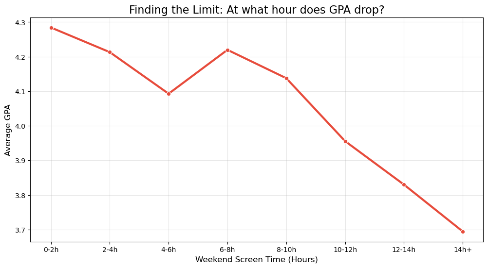
Average GPA by Screen Time Bucket:
Screen_Bin
0-2h      4.284167
2-4h      4.212963
4-6h      4.092826
6-8h      4.219706
8-10h     4.137647
10-12h    3.955625
12-14h    3.830000
14h+      3.694444
Name: GPA, dtype: float64


/var/folders/d8/4k3q_2wd4nv9gmh9ch_b79jr0000gn/T/ipykernel_98634/2438005933.py:28: FutureWarning: The default of observed=False is deprecated and will be changed to True in a future version of pandas. Pass observed=False to retain current behavior or observed=True to adopt the future default and silence this warning.
  print(df.groupby('Screen_Bin')['GPA'].mean())
# 1. Round Sleep to nearest hour for grouping
df['Sleep_Rounded'] = df['Sleep_Hours'].round()

# 2. Visualize the Curve
plt.figure(figsize=(12, 6))
sns.lineplot(
    data=df,
    x='Sleep_Rounded',
    y='GPA',
    marker='o',
    linewidth=3,
    color='#2ecc71', # Green because sleep is good
    errorbar=None
)

plt.title('Finding the Sweet Spot: How many hours of Sleep?', fontsize=16)
plt.ylabel('Average GPA', fontsize=12)
plt.xlabel('Sleep Duration (Hours)', fontsize=12)
plt.xticks(range(4, 11)) # Show 4, 5, 6... 10
plt.grid(True, alpha=0.3)
plt.show()

# 3. Print the Numbers
print("Average GPA by Sleep Hours:")
print(df.groupby('Sleep_Rounded')['GPA'].mean())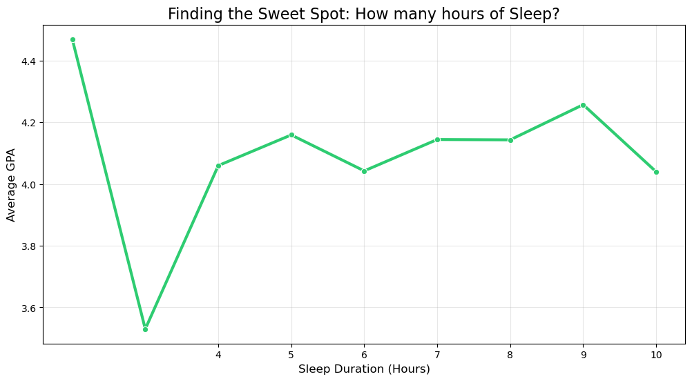
Average GPA by Sleep Hours:
Sleep_Rounded
2.0     4.470000
3.0     3.530000
4.0     4.060000
5.0     4.159412
6.0     4.042857
7.0     4.144545
8.0     4.143514
9.0     4.257500
10.0    4.040000
Name: GPA, dtype: float64
# 1. Define Order
order = ['Ни одного', '1-2', '2-3', 'Более 3 раз']

# 2. Visualize
plt.figure(figsize=(10, 6))
sns.lineplot(
    data=df,
    x='Training_Freq',
    y='GPA',
    marker='o',
    linewidth=3,
    color='#3498db', # Blue
    errorbar=None
)

plt.title('Finding the Sweet Spot: Training Frequency', fontsize=16)
plt.ylabel('Average GPA', fontsize=12)
plt.xlabel('Training Frequency', fontsize=12)
plt.grid(True, alpha=0.3)
plt.show()